1 Billion Classifications


You’ve optimized your model. Your pipeline is running smoothly. But now, your cloud bill has skyrocketed. Running 1B+ classifications or embeddings per day isn’t just a technical challenge—it’s a financial one. How do you process at this scale without blowing your budget? Whether you're running large-scale document classification or bulk embedding pipelines for Retrieval-Augmented Generation (RAG), you need cost-efficient, high-throughput inference to make it feasible, and you get that from having a well optimized configuration.
These tasks often use encoder models, which are much smaller than modern LLMs, but at the 1B+ inference request scale it's still quite a non-trivial task. Just to be clear, that's English Wikipedia 144x over. I haven’t seen much information on how to approach this with cost in mind and I want to tackle that. This blog breaks down HOW to calculate cost and latency for large scale classification and embedding. We’ll analyze different model architectures, benchmark costs across hardware choices, and give you a clear framework for optimizing your own setup. Additionally we should be able to build some intuition if you don't feel like going through the process yourself.
You might have a couple questions:
- What is the cheapest configuration to solve my task for 1B inputs? (Batch Inference)
- How can I do that while also considering latency? (Heavy Usage)
Here is the code to make it happen: https://github.com/datavistics/encoder-analysis
tl;I'm not gonna reproduce this, tell me what you found;dr
With this pricing I was able to get this cost:
| Use Case | Classification | Embedding | Vision-Embedding |
|---|---|---|---|
| Model | lxyuan/distilbert-base-multilingual-cased-sentiments-student | Alibaba-NLP/gte-modernbert-base | vidore/colqwen2-v1.0-merged |
| Data | tyqiangz/multilingual-sentiments | sentence-transformers/trivia-qa-triplet | openbmb/RLAIF-V-Dataset |
| Hardware Type | nvidia-L4 ($0.8/hr) |
nvidia-L4 ($0.8/hr) |
nvidia-L4 ($0.8/hr) |
| Cost of 1B Inputs | $253.82 | $409.44 | $44,496.51 |
Approach
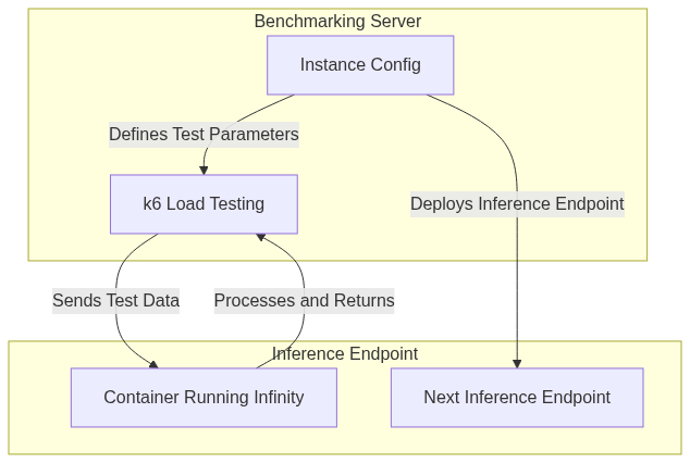
To evaluate cost and latency we need 4 key components:
- Hardware options: A variety of hardware to compare costs
- Deployment Facilitator: A way to deploy models with settings of our choice
- Load Testing: A way of sending requests and measuring the performance
- Inference Server: A way to run the model efficiently on the hardware of choice
I’ll be leveraging Inference Endpoints for my Hardware Options, as it allows me to choose from a wide range of hardware choices. Do note you can replace that with your GPUs of choice/consideration. For the Deployment Facilitator I'll be using the ever so useful Hugging Face Hub Library which allows me to programmatically deploy models easily.
For the Inference Server I’ll also be using Infinity which is an amazing library for serving encoder based models (and more now!). I’ve already written about TEI, which is another amazing library. You should definitely consider TEI when approaching your use-case, though this blog focuses on methodology rather than framework comparisons. Infinity has a number of key strengths, like serving multimodal embeddings, targeting different hardware (AMD, Nvidia, CPU and Inferentia) and running any new models that contain remote code that have not been integrated into huggingface’s transformer library. The most important of these to me is that most models are compatible by default.
For Load Testing I'll be using k6 from Grafana which is an open-source load testing tool written in go with a javascript interface. It’s easily configurable, has high performance, and has low overhead. It has a lot of built-in executors that are super useful. It also pre-allocates Virtual Users (VUs), which can be much more realistic than throwing some testing together yourself.
I'll go through 3 use-cases that should cover a variety of interesting points:
| Use-case | Model | Base Architecture | Parameter Count | Interest |
|---|---|---|---|---|
| Classification (Text) | lxyuan/distilbert-base-multilingual-cased-sentiments-student | DistilBertForSequenceClassification | 135M | The distilled architecture is small/fast and ideal for some. |
| Embedding | Alibaba-NLP/gte-modernbert-base | ModernBertModel | 149M | Uses ModernBERT, and can be super fast. Extendable for long-contexts too. |
| Vision-Embedding | vidore/colqwen2-v1.0-merged | ColQwen2 | 2.21B | ColQwen2 can provide unique insights in a ColBERT-Style retrieval of VLMs |
Optimization
Optimization is a tricky issue, as there is a lot to consider. At a high level, I want to sweep across important load testing parameters and find what works best for a single GPU, as most encoder models will fit in a single GPU. Once we have a baseline of cost for a single GPU, the number of GPUs and throughput can be scaled horizontally by increasing the number of replica GPUs.
Setup
For each use-case this is the high-level flow I’ll use:
Since you have the code, feel free to adjust any part of this to your:
- GPUs
- Deployment process
- Experimentation Framework
- Etc
You won’t hurt my feelings.
Load Testing Parameters
VUs and Batch Size are important because these influence how well we take advantage of all the compute available in the GPU. A large enough Batch Size makes sure we are fully utilizing the Streaming Multiprocessors and VRAM. There are scenarios where we have VRAM left over but there is a bandwidth cost that prevents throughput from increasing. So experimentation can help us. VUs allow us to make sure we are fully utilizing the batch size we have available.
These are the main parameters I'll be testing:
INFINITY_BATCH_SIZE- This is how many documents will make a forward pass in the batch in the model
- Too low and we won't be utilizing the GPU
- Too high and the GPU can't handle the large input
VUs- This is the number of Virtual Users simulating parallel client requests that is sent to K6
- It can be hard to simulate a large number of users, and each machine will vary.
- GPUs
- We have a variety of GPUs available on Inference Endpoints
- I prioritized those with the best performance/cost ratio
- CPUs
- I omitted these since Nvidia-T4s are so cheap that CPUs didn’t seem appealing upon light testing. I left some code to test this if a user is interested though!
Depending on your model you might want to consider:
- Which Docker image you are using. [
'michaelf34/infinity:0.0.75-trt-onnx','michaelf34/infinity:0.0.75']- There are a number of Infinity Images that can support different backends. You should consider which ones are most applicable to your hardware/model/configuration.
INFINITY_COMPILEwhether or not you want to usetorch.compile()docsINFINITY_BETTERTRANSFORMERwhether or not you want torch to use Better Transformer
K6
K6 is great because it allows you to pre-allocate VUs and prevent some insidious bugs. It's quite flexible in how you are sending requests. I decided to use it in a specific way.
When I'm calling a k6 experiment, I mainly want to know what the throughput and average latency is for the requests, and have a few sanity checks for the load testing parameters I have chosen. I also want to do a sweep which means many experiments.
I use the shared-iterations executor (docs) which means K6 shares iterations between the number of VUs. The test ends once k6 executes all iterations. This allows me to have a reasonable time-out, but also put through enough requests to have a decent confidence that I can discriminate between load testing parameters choices in my sweep. In contrast to other executors, this allows me to be confident that I'm simulating the client working as hard as possible per VU which should show me what the cheapest option is.
I use 10_000 requests† and have a max experiment time of 1 min. So if 10_000 requests aren’t finished by 1 minute, then that experiment is over.
export const options = {
    scenarios: {
        shared_load_test: {
            executor: 'shared-iterations',
            vus: {{ pre_allocated_vus }},
            iterations: 10000,
            maxDuration: '1m',
        },
    },
};
Stats
- P95†† and Average Latency
- Throughput
Sanity Checks
- Accuracy (Classification only)
- Test Duration
- Successful Requests
- Format validation
† I use less max requests for the Vision Embeddings given that the throughput is much lower and images are heavy.
†† P95 means that 95% of requests complete within this time. It represents the worst-case latency for most users.
Orchestration
You can find the 3 notebooks that put the optimization workflow together here:
The main purpose was to get my experiments defined, launch the correct Inference Endpoint with the right parameters, and launch k6 with the right parameters to test the endpoint.
I made a couple design choices which you may want to think through to see if they work for you:
- I do an exponential increase of VUs then a binary search to find the best value
- I don’t treat the results as exactly repeatable
- If you run the same test multiple times you will get slightly different results
- I used an improvement threshold of 2% to decide if I should keep searching
Classification
Introduction
Text Classification can have a variety of use-cases at scale, like Email Filtering, Toxicity Detection in pre-training datasets, etc. The OG classic architecture was BERT, and quickly many other architectures came about. Do note that in contrast to popular decoder models, these need to be fine-tuned on your task before using them. Today I think the following architectures† are the most notable:
- DistilBERT
- Good task performance, Great Engineering performance
- It made some architectural changes from OG Bert and is not compatible for classification with TEI
- DeBERTa-v3
- Great task performance
- Very slow engineering performance†† as its unique attention mechanism is hard to optimize
- ModernBERT
- Uses Sequence Packing and Flash-Attention-2
- Great task performance and great engineering performance††
† Do note that for these models, you typically need to fine-tune this on your data to perform well
†† I'm using “Engineering performance” to denote anticipated latency/throughput
Experiment
| Category | Values |
|---|---|
| Model | lxyuan/distilbert-base-multilingual-cased-sentiments-student |
| Model Architecture | DistilBERT |
| Data | tyqiangz/multilingual-sentiments (text col) Avg of 100 token (min of 50), multiple languages |
| Hardware | nvidia-L4 ($0.8/hr) nvidia-t4 ($0.5/hr) |
| Infinity Image | trt-onnx vs default |
batch_size |
[16, 32, 64, 128, 256, 512, 1024] |
vus |
32+ |
I chose DistilBERT to focus on as it’s a great lightweight choice for many applications. I compared 2 GPUs, nvidia-t4 and nvidia-l4 as well as 2 Infinity Docker Images.
Results
You can see the results in an interactive format here or in the space embedded below in the Analysis section. This is the cheapest configuration across the experiments I ran:
| Category | Best Value |
|---|---|
| Cost of 1B Inputs | $253.82 |
| Hardware Type | nvidia-L4 ($0.8/hr) |
| Infinity Image | default |
batch_size |
64 |
vus |
448 |
Embedding
Introduction
Text Embeddings are a loose way of describing the task of taking a text input and projecting it into a semantic space where close points are similar in meaning and distant ones are dissimilar (example below). This is used heavily in RAG and is an important part of AI search (which some are fans of).
There are a large number of architectures which are compatible, and you can see the most performant ones in the MTEB Leaderboard.
Experiment
ModernBERT is the most exciting encoder release since DeBERTa back in 2020. It has all the ahem modern tricks built into an old and familiar architecture. It makes for an attractive model to experiment with as it's much less explored than other architectures and has a lot more potential. There are a number of improvements in speed and performance, but the most notable for a user is likely the 8k context window. Do check out this blog for a more thorough understanding.
It's important to note that Flash Attention 2 will only work with more modern GPUs due to the compute capability requirement, so I opted to skip the T4 in favor of the L4. An H100 would also work really well here for the heavy hitters category.
| Category | Values |
|---|---|
| Model | Alibaba-NLP/gte-modernbert-base |
| Model Architecture | ModernBERT |
| Data | sentence-transformers/trivia-qa-triplet (positive col) Avg of 144 tokens std dev of 14. |
| Hardware | nvidia-L4 ($0.8/hr) |
| Infinity Image | default |
batch_size |
[16, 32, 64, 128, 256, 512, 1024] |
vus |
32+ |
Results
You can see the results in an interactive format here. This is the cheapest configuration across the experiments I ran:
| Category | Best Value |
|---|---|
| Cost of 1B Inputs | $409.44 |
| Hardware Type | nvidia-L4 ($0.8/hr) |
| Infinity Image | default |
batch_size |
32 |
vus |
256 |
Vision Embedding
Introduction
ColQwen2 is a Visual Retriever which is based on the Qwen2-VL-2B-Instruct and uses ColBERT style multi-vector representations of both text and images. We can see that it has a complex architecture compared to the encoders we explored above.

There are a number of use-cases which might benefit from this at large scale like, e-commerce search, multi-modal recommendations, enterprise multi-modal RAG, etc
ColBERT style is different than our previous embedding use-case since it breaks the input into multiple tokens and returns a vector for each instead of 1 vector for the input. You can find an excellent tutorial from Jina AI here.This can lead to superior semantic encoding and better retrieval, but is also slower, and more expensive.
I'm excited for this experiment as it explores 2 lesser known concepts, vision embeddings and ColBERT style embeddings†. There are a few things to note about ColQwen2/VLMs:
- 2B is ~15x bigger than the other models we looked at in this blog
- ColQwen2 has a complex architecture with multiple models including a decoder which is slower than an encoder
- Images can easily consume a lot of tokens
- API Costs:
- Sending images over an API is slower than sending text.
- You will further encounter larger egress costs if you are on a cloud
†Do check out this more detailed blog if this is new and interesting to you.
Experiment
I wanted to try a small and modern GPU like the nvidia-l4 since it should be able to fit the 2B param model but also scale well since it's cheap. Like the other embedding model, I'm varying batch_size and vus.
| Category | Values |
|---|---|
| Model | vidore/colqwen2-v1.0-merged |
| Model Architecture | ColQwen2 |
| Data | openbmb/RLAIF-V-Dataset (image col) Most images are ~600x400 at 4MB |
| Hardware | nvidia-L4 ($0.8/hr) |
| Infinity Image | default |
batch_size |
[1, 2, 4, 8, 16] |
vus |
1+ |
Results
You can see the results in an interactive format here. This is the cheapest configuration across the experiments I ran:
| Category | Best Value |
|---|---|
| Cost of 1B Inputs | $44,496.51 |
| Hardware Type | nvidia-l4 |
| Infinity Image | default |
batch_size |
4 |
vus |
4 |
Analysis
Do check out the detailed analysis in this space (derek-thomas/classification-analysis) for the classification use-case (hide side-bar and scroll down for the charts):
Conclusion
Scaling to 1B+ classifications or embeddings per day is a non-trivial challenge, but with the right optimizations, it can be made cost-effective. From my experiments, a few key patterns emerged:
- Hardware Matters – NVIDIA L4 ($0.80/hr) consistently provided the best balance of performance and cost, making it the preferred choice over T4 for modern workloads. CPUs were not competitive at scale.
- Batch Size is Critical – The sweet spot for batch size varies by task, but in general, maximizing batch size without hitting GPU memory and bandwidth limits is the key to efficiency. For classification, batch size 64 was optimal; for embeddings, it was 32.
- Parallelism is Key – Finding the right number of Virtual Users (VUs) ensures GPUs are fully utilized. An exponential increase + binary search approach helped converge on the best VU settings efficiently.
- ColBERT style Vision Embeddings are Expensive – At over $44,000 per 1B embeddings, image-based retrieval is 2 orders of magnitude costlier than text-based tasks.
Your data, hardware, models, etc might differ, but I hope you find some use in the approach and code provided. The best way to get an estimate is to run this on your own task with your own configurations. Let's get exploring!
Special thanks to andrewrreed/auto-bench for some inspiration, Michael Feil for creating Infinity. Also thanks to Pedro Cuenca, Erik Kaunismaki, and Tom Aarsen for helping me review.
References
- https://towardsdatascience.com/exploring-the-power-of-embeddings-in-machine-learning-18a601238d6b
- https://yellow-apartment-148.notion.site/AI-Search-The-Bitter-er-Lesson-44c11acd27294f4495c3de778cd09c8d
- https://jina.ai/news/what-is-colbert-and-late-interaction-and-why-they-matter-in-search/
Appendix
Sanity Checks
It's important to scale sanity checks as your complexity scales. Since we are using subprocess and jinja to then call k6 I felt far from the actual testing so I put a few checks in place.
Task Performance
The goal of task performance is that for a specific configuration we are performing similarly to what we expect. Task Performance will have different meanings across tasks. For classification I chose accuracy, and for embeddings I skipped it. We could look at average similarity and other similar metrics. It gets a bit more complex with ColBERT style since we are getting many vectors per request.
Even though 58% isn't bad for some 3 class classification tasks, it's irrelevant. The goal is to make sure that we are getting the expected task performance. If we see a significant change (increase or decrease) we should be suspicious and try to understand why.
Below is a great example from the classification use-case since we can see an extremely tight distribution and one outlier. Upon further investigation the outlier is due to a low amount of requests sent.

You can see the interactive results visualized by nbviewer here:
Failed Requests Check
We should expect to see no failed requests as Inference Endpoints has a queue to handle extra requests. This is relevant for all 3 use-cases: Classification, Embedding, and Vision Embedding.
sum(df.total_requests - df.successful_requests) allows us to see if we had any failed requests.
Monotonic Series - Did we try enough VUs?
As described above we are using a nice strategy of using exponential increases and then a binary search to find the best number of VUs. But how do we know that we tried enough VUs? What if we tried a higher amount of VUs and throughput kept increasing? If that's the case then we would see a monotonically increasing relationship between VUs and Throughput and we would need to run more tests.
You can see the interactive results visualized by nbviewer here:
Embedding Size Check
When we request an embedding it makes sense that we would always get back an embedding of the same size as specified by the model type. You can see the checks here:
- Embedding
- Vision Embedding (inner embedding)
ColBERT Embedding Count
We are using a ColBERT style model for Vision Embedding which means we should be getting multiple vectors per image. It's interesting to see the distribution of these as it allows us to check for anything unexpected and to get to know our data. To do so I stored the min_num_vectors, avg_num_vectors, max_num_vectors, in the experiments.
We should expect to see some variance in all 3, but it’s ok that min_num_vectors and max_num_vectors have the same value across experiments.
You can see the check here:
Cost Analysis
Here is a short description, but you can get a more detailed interactive experience in the space: derek-thomas/classification-analysis
Best Image by Cost Savings
For the classification use-case we looked at 2 different Infinity Images, default and trt-onnx. Which one was better? It's best if we can compare these across the same settings (GPU, batch_size, VUs). We can simply group our results by those settings and then see which one was cheaper.

Cost vs Latency
This is a key chart as for many use-cases there is a maximum latency that a user can experience. Usually if we allow the latency to increase we can increase throughput creating a trade-off scenario. That's true in all the use-cases I've looked at here. Having a pareto curve is great to help visualize where that tradeoff is.
Cost vs VUs and Batch Size Contour Plots
Lastly it's important to build intuition on what is happening when we try these different settings. Do we get beautiful idealized charts? Do we see unexpected gradients? Do we need more exploration in a region? Could we have issues in our setup like not having an isolated environment? All of these are good questions and some can be tricky to answer.
The contour plot is built by interpolating intermediate points in a space defined by the 3 dimensions. There are a couple phenomena that are worth understanding:
- Color Gradient: Shows the cost levels, with darker colors representing higher costs and lighter colors representing lower costs.
- Contour Lines: Represent cost levels, helping identify cost-effective regions.
- Tight clusters: (of contour lines) indicate costs changing rapidly with small adjustments to batch size or VUs.
We can see a complex contour chart with some interesting results from the classification use-case:

But here is a much cleaner one from the vision-embedding task:

Infinity Client
For actual usage, do consider using the infinity client. When we are benchmarking it's good practice to use k6 to know what’s possible. For actual usage, use the official lib, or something close for a few benefits:
- Base64 means smaller payloads (faster and cheaper)
- The maintained library should make development cleaner and easier
- You have inherent compatibility which will make development faster
You also have OpenAI lib compatibility with the Infinity backend as another option.
As an example vision-embeddings can be accessed like this:
pip install infinity_client && python -c "from infinity_client.vision_client import InfinityVisionAPI"
Other Lessons Learned
- I tried deploying multiple models on the same GPU but didn’t see major improvements despite having leftover VRAM and GPU processing power left, this is likely due to the bandwidth cost of processing a large batch
- Getting K6 to work with images was a headache until I learned about SharedArrays
- Image Data can be super cumbersome to work with
- The key to debugging K6 when you are generating scripts is to manually run K6 and look at the output.
Future Improvements
- Have the tests run in parallel while managing a global max of
VUswould save a lot of time - Look at more diverse datasets and see how that impacts the numbers